Example 05: Density currents with cosine shaped bottom
Purpose
To calculate the density currents in a cosine shaped bottom tank.
Creation of calculation grid and setting initial conditions
Create the calculation grid using [Grid] [Select Algorithm to Create Grid] and then select [Gird Generator for Nays2DV] in select grid creating algorithm window.
Give channel bottom shape parameters as shown in Figure 70. Since the bottom profile data is not not available, select how to set longitudinal bed profile as automatically. If longitudinal bed profile data available select manually and give the data for longitudinal bed profile location.
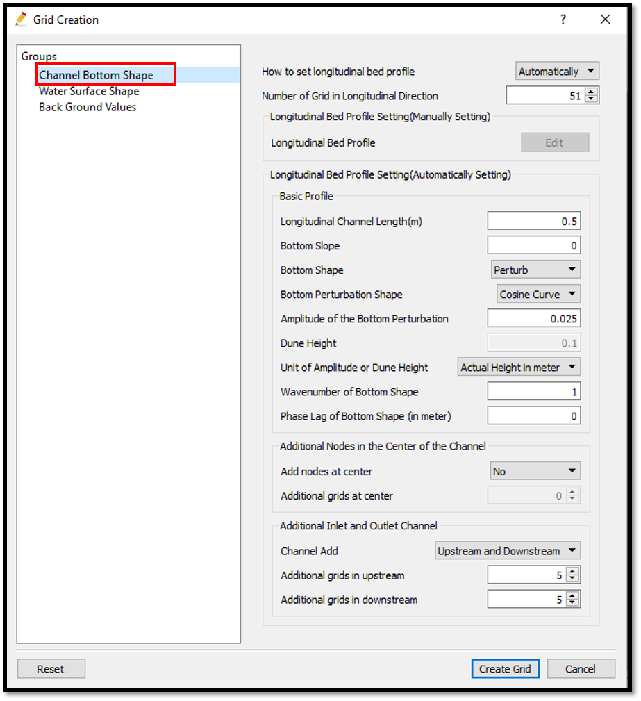
Figure 70 : Channel shape parameters
For this example, give bottom shape as perturbed and perturbation shape as cosine curve. Amplitude of the bottom perturbation is 0.025. Unit of amplitude or dune height is actual height in meter. Wave number of bottom shape is 1. Phase lag of bottom shape is 0.
Give water surface sape parameters as as shown in Figure 71.
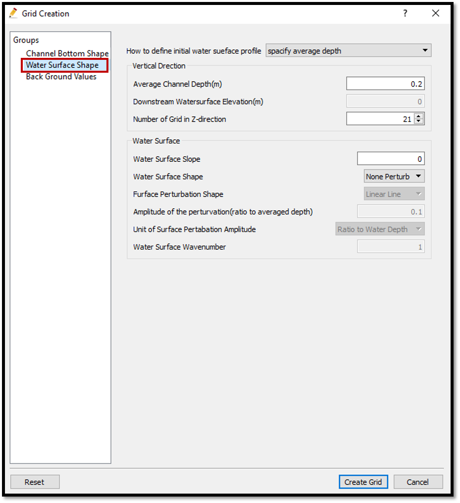
Figure 71 : Bottom and surface parameters
Give background values as shown in Figure 72.
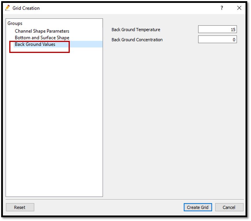
Figure 72 : Background values
For the background values of temperature and initial concentration, background temperature is 15 and initial concentration is 0.
Now create the grid.
A confirmation message will be asked to map geographic data to the grid. Select yes. However, later have to again map the attributes if new polygons are added etc. Now add the initial concentration, that is different to background initial concentration.
Add a polygon to initial concentration by right clicking on [Initial Concentration] and [Add] [Polygon]. Now draw the polygon as shown in Figure 73. Add the initial concentration value of 0.03.
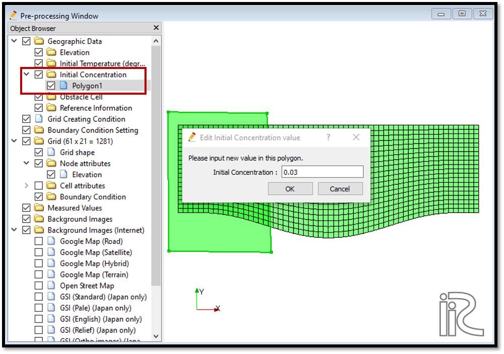
Figure 73 : Setting Initial concentration
Then, map the initial concentration value to the grid using, [Grid] [Attributes mapping] [Execute] and tick on initial concentration on the attribute mapping window as shown in Figure 74.
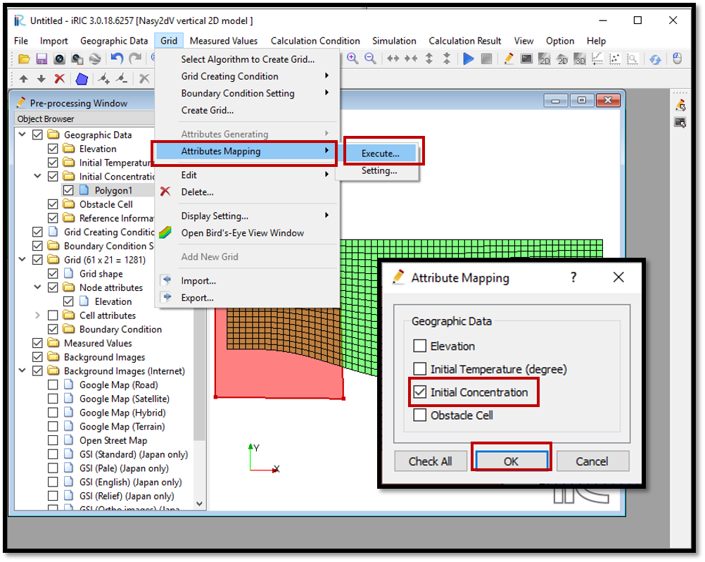
Figure 74 : Attributes mapping
Now the initial concentration is mapped to the grid. Now save the project with [File] [Save project as .ipro].
Setting the calculation conditions and simulation
Give the calculation conditions with, [Calculation Condition] [Settings]
Give computational parameters as shown in Figure 75.
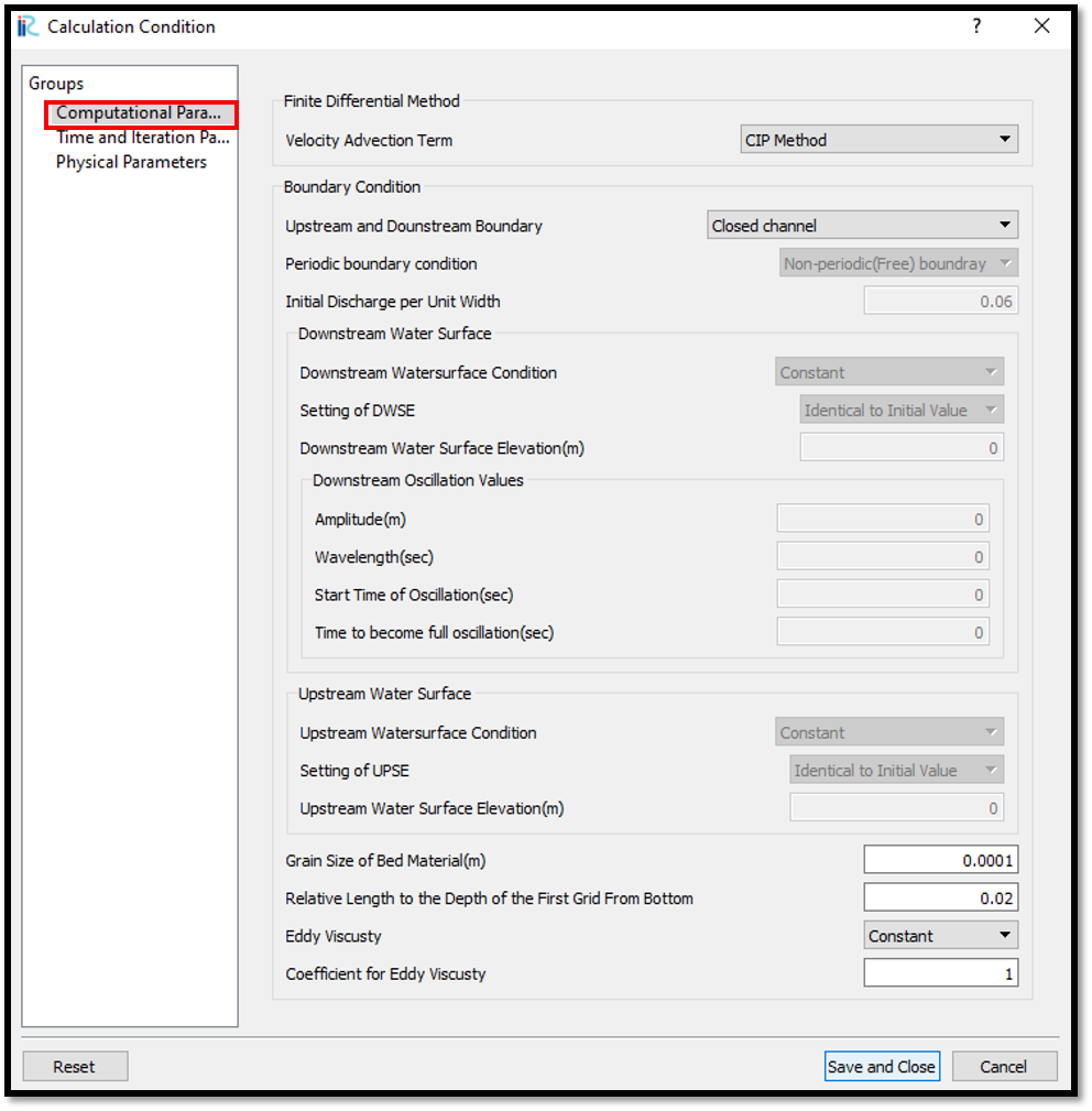
Figure 75 : Computational parameters
Give time and iteration parameters as shown in Figure 76.
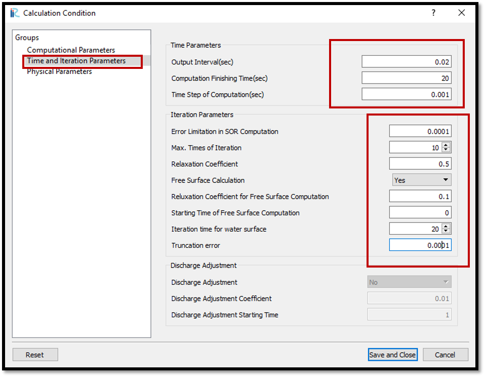
Figure 76 : Time and iteration parameters
Adjust time parameters as output interval=0.02sec Computation finishing time=20s Time step=0.001 Free surface calculation = yes Relaxation coefficient for free surface computation=0.1 Iteration time for water surface=20
Give physical parameters as shown in Figure 77.
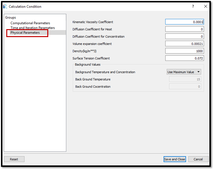
Figure 77 : Physical parameters
After setting the calculation conditions, save the project by clicking on save tab. Now start simulation by, [Simulation] [Run]. Simulation will start and after some time it will finish showing the message the solver finished the calculation.
Visualization of results
Open 2D post processing window by selecting, [Calculation Results] [Open new 2D Post-Processing Window].
Select any parameter in [Object Browser], [iRIC Zone].
In this example select, concentration by ticking on [iRIC Zone] [Scaler] and [Concentration]. Properties of visual figure can be adjusted by right clicking on [Concentration] and selecting [Property].
Adjust the scaler settings as shown in Figure 78.
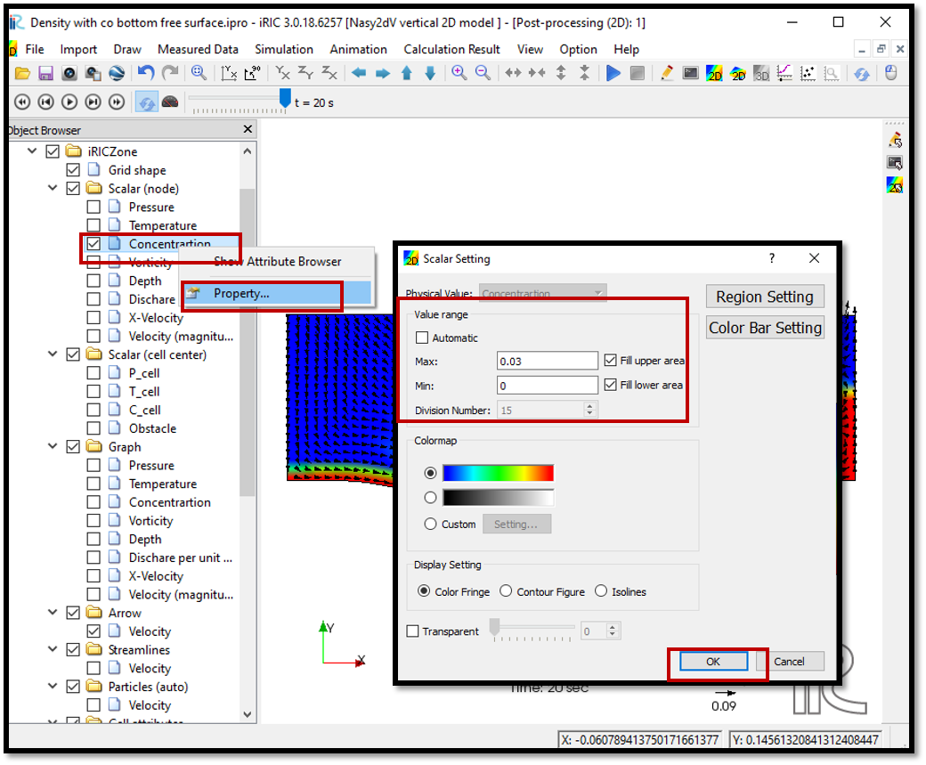
Figure 78 : Scaler setting .
To set the currents movements direction, select [Velocity] in object browser by ticking on [iRIC Zone] [Arrow] and [Velocity].
Adjust the sizes of velocity vectors by right clicking on [Arrow] and selecting [Property] as shown in Figure 79.
Figure 79 : Arrow setting
The Figure 80 is the result of the above process.

Figure 80 : Concentration & velocity vector plot